!python -m pip install --upgrade pip -q
!pip install geopandas -q

import seaborn as sns
import matplotlib.pyplot as plt
import numpy as np

# Define file paths
gini_file_path = r"C:\Users\11\Desktop\Python\Python Project\Global Inequlity Analysis\Gini Index.xlsx"
gdp_file_path = r"C:\Users\11\Desktop\Python\Python Project\Global Inequlity Analysis\NationalGDP.xls"

# Read the Excel files
df = pd.read_excel(gini_file_path, engine="openpyxl")
GDP = pd.read_excel(gdp_file_path, engine="xlrd")

# Clean column names by stripping spaces and replacing inner spaces with underscores
GDP.columns = GDP.columns.str.strip().str.replace(r'\s+', '_', regex=True)
df.columns = df.columns.str.strip().str.replace(r'\s+', '_', regex=True)

# Pivot the Gini Index table so that each country's yearly values become columns
pivot_df = df.pivot_table(values="Gini_Index", index=['Country', 'ISO-3_Code'], columns="Year")

# Select the years 2013 to 2022
IEQ_10 = pivot_df[[2013, 2014, 2015, 2016, 2017, 2018, 2019, 2020, 2021, 2022]]
GDP_10 = GDP[['Country_Code', '2013', '2014', '2015', '2016', '2017', '2018', '2019', '2020', '2021', '2022']]

# Compute the median Gini Index (IEQ value) for each country
IEQ_10_Median = IEQ_10.median(axis=1).reset_index()

# Compute the mean GDP across the selected years for each country
GDP_10_Mean = GDP_10.set_index('Country_Code').mean(axis=1).reset_index()

# Rename ISO-3_Code to Country_Code in the IEQ dataframe for merging
IEQ_10_Median.rename(columns={"ISO-3_Code": "Country_Code"}, inplace=True)

# Merge the two datasets on Country_Code
Co_IEQ_GDP = IEQ_10_Median.merge(GDP_10_Mean, on='Country_Code', suffixes=('_ieq', '_gdp'))

# For clarity, rename the merged numeric columns to '0_ieq' and '0_gdp'
# The merged DataFrame typically ends up with the new GDP column as the third column.
Co_IEQ_GDP.rename(columns={Co_IEQ_GDP.columns[2]: '0_ieq', Co_IEQ_GDP.columns[3]: '0_gdp'}, inplace=True)

print(Co_IEQ_GDP.head())

# Drop rows with non-finite values in '0_gdp' or '0_ieq'
Co_IEQ_GDP = Co_IEQ_GDP[np.isfinite(Co_IEQ_GDP['0_gdp']) & np.isfinite(Co_IEQ_GDP['0_ieq'])]

# Sort the DataFrame by '0_gdp' (mean GDP) in ascending order
Co_IEQ_GDP = Co_IEQ_GDP.sort_values(by='0_gdp', ascending=True)

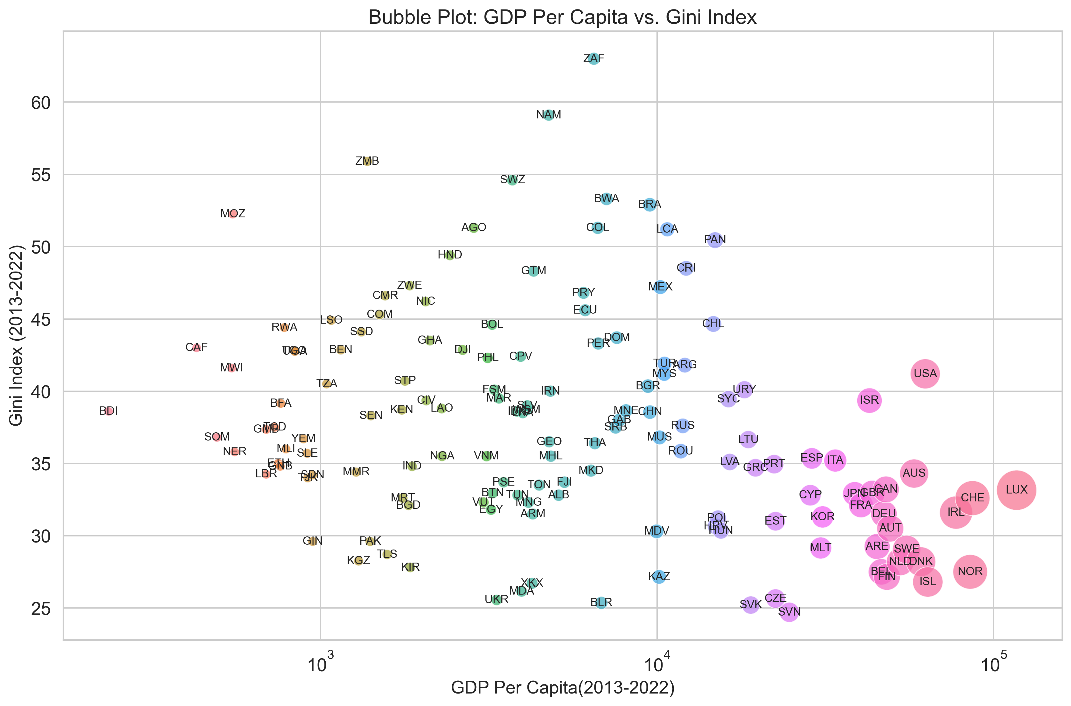
# Set up the bubble plot figure
plt.figure(figsize=(12, 8))
sns.set_theme(style="whitegrid", palette="muted", font="sans-serif", font_scale=1.3)
plt.figure(figsize=(12, 8), dpi=300)
# Create the bubble plot:
scatter = sns.scatterplot(
    data=Co_IEQ_GDP,
    x='0_gdp',          # x-axis: mean GDP
    y='0_ieq',          # y-axis: median Gini Index
    size='0_gdp',       # Bubble size based on mean GDP (you can change this if desired)
    sizes=(50, 1000),   # Adjust bubble size range
    alpha=0.7,          # Transparency for bubbles
    hue='Country',
    legend=False,
)

# Annotate each bubble with the Country_Code
for _, row in Co_IEQ_GDP.iterrows():
    # Only annotate if both values are finite
    if np.isfinite(row['0_gdp']) and np.isfinite(row['0_ieq']):
        plt.text(row['0_gdp'], row['0_ieq'], row['Country_Code'],
                 fontsize=9, ha='center', va='center')
plt.xscale('log')
# Customize the plot
plt.title("Bubble Plot: GDP Per Capita vs. Gini Index", fontsize=16)
plt.xlabel("GDP Per Capita(2013-2022)", fontsize=14)
plt.ylabel("Gini Index (2013-2022)", fontsize=14)
plt.grid(True)
plt.tight_layout()

# Display the plot
plt.show()

import geopandas as gpd
import pandas as pd
import matplotlib.pyplot as plt

# Load world map data
world = gpd.read_file(r"C:\Users\11\Desktop\Python\Python Project\Global Inequlity Analysis\110m_cultural\ne_110m_admin_0_countries.shp")

# Load GINI Index data
GINI = pd.read_excel(r"C:\Users\11\Desktop\Python\Python Project\Global Inequlity Analysis\Gini Index.xlsx")

# Strip spaces from column names
GINI.columns = GINI.columns.str.strip()

# Ensure 'Year' is numeric
GINI['Year'] = pd.to_numeric(GINI['Year'], errors='coerce')

# Filter data for years 2013-2022 and calculate the median
GINI_filtered = GINI[(GINI['Year'] >= 2013) & (GINI['Year'] <= 2022)]
Pivot_GINI = GINI_filtered.pivot_table(values="Gini Index", index=['Country', 'ISO-3 Code'], aggfunc='median')

# Reset index so 'ISO-3 Code' is no longer part of the index
Pivot_GINI.reset_index(inplace=True)

# Rename median column
GINI_median = Pivot_GINI.rename(columns={"Gini Index": 'GINI_Median'})

# Merging datasets
merged_gini = world.set_index('SOV_A3').join(GINI_median.set_index('ISO-3 Code'))

# Filter out invalid values
filtered_merged_gini = merged_gini[merged_gini['GINI_Median'] > 0]

# Plot the GINI Index map
fig, ax = plt.subplots(1, 1, figsize=(15, 10))
filtered_merged_gini.plot(column='GINI_Median', ax=ax, legend=True, cmap="RdYlGn_r",
                           legend_kwds={'label': "Median GINI Index (2013-2022) by Country", 'orientation': "horizontal"})
plt.show()

import pandas as pd
import matplotlib.pyplot as plt
import matplotlib.lines as mlines

# Load GINI data
GINI = pd.read_excel(r"C:\Users\11\Desktop\Python\Python Project\Global Inequlity Analysis\Gini Index.xlsx")

# Strip spaces from column names
GINI.columns = GINI.columns.str.strip()

# Ensure 'Year' is numeric
GINI['Year'] = pd.to_numeric(GINI['Year'], errors='coerce')

# Filter data for years 2013-2022 and calculate the median
GINI_filtered = GINI[(GINI['Year'] >= 2013) & (GINI['Year'] <= 2022)]
Pivot_GINI = GINI_filtered.pivot_table(values="Gini Index", index=['Country', 'ISO-3 Code'], aggfunc='median')

# Reset index so 'ISO-3 Code' is no longer part of the index
Pivot_GINI.reset_index(inplace=True)

print(Pivot_GINI.head())

# Sort and select top/bottom 30
sorted_GINI = Pivot_GINI.sort_values('Gini Index', ascending=False)
top_30_GINI = sorted_GINI.head(30)
bottom_30_GINI = sorted_GINI.tail(30)

def highlight_top3(rank):
    if rank == 1:
        return 'gold'
    elif rank == 2:
        return 'silver'
    elif rank == 3:
        return 'brown'
    else:
        return 'skyblue'

# Function to create lollipop chart
def lollipop_chart(data, title):
    # Sort data
    sorted_data = data.sort_values('Gini Index', ascending=False)

    # Create base figure and axis
    fig, ax = plt.subplots(figsize=(12, 12))

    # Lollipop lines
    ax.vlines(x=sorted_data['Country'], ymin=0, ymax=sorted_data['Gini Index'], color='gray', alpha=0.6)

    # Lollipop heads
    ax.scatter(sorted_data['Country'], sorted_data['Gini Index'], color=[highlight_top3(rank) for rank in range(1, len(data)+1)], s=75, alpha=0.6)

    # Title & grid
    ax.set_title(title, fontdict={'size':15})
    ax.grid(linestyle='--', alpha=0.6)
    ax.set_xlabel('Country')
    ax.set_ylabel('Gini Index (Median 2013-2022)')
    plt.xticks(rotation=90)

    # Display
    plt.gca().invert_xaxis()  # For top ranks to appear on the left side.
    plt.show()

# Create lollipop charts for top and bottom 30 countries
lollipop_chart(bottom_30_GINI, 'Top 30 Countries that have the lowest Gini Index (Median 2013-2022)')
lollipop_chart(top_30_GINI, 'Bottom 30 Countries that have the lowest Gini Index (Median 2013-2022)')

import geopandas as gpd
import pandas as pd
import matplotlib.pyplot as plt

# Load world map data
world = gpd.read_file(r"C:\Users\11\Desktop\Python\Python Project\Global Inequlity Analysis\110m_cultural\ne_110m_admin_0_countries.shp")

# Load HDI data
HDI = pd.read_excel(r"C:\Users\11\Desktop\Python\Python Project\Global Inequlity Analysis\Human development index (HDI).xlsx")

# Strip spaces from column names
HDI.columns = HDI.columns.str.strip()


# Ensure 'Year' is numeric
HDI['Year'] = pd.to_numeric(HDI['Year'], errors='coerce')

# Pivot Table
Pivot_HDI = HDI.pivot_table(values="Human development index (HDI)", index=['Country', 'ISO-3 Code'], columns="Year")

# Reset index so 'ISO-3 Code' is no longer part of the index
Pivot_HDI.reset_index(inplace=True)

# Extract HDI for 2022
if 2022 in Pivot_HDI.columns:  # Ensure 2022 data exists
    HDI_2022 = Pivot_HDI[['ISO-3 Code', 2022]].rename(columns={2022: 'HDI_2022'})
else:
    raise ValueError("HDI data for 2022 is not available in the dataset.")

# Print first rows to verify

# Merging datasets
merged = world.set_index('SOV_A3').join(HDI_2022.set_index('ISO-3 Code'))

# Print to verify the merge


# Filter out countries with HDI rank of 0
filtered_merged = merged[merged['HDI_2022'] > 0]

fig, ax = plt.subplots(1, 1, figsize=(15, 10))
filtered_merged.plot(column='HDI_2022', ax=ax, legend=True, cmap="RdYlGn",
                    legend_kwds={'label': "HDI Rank by Country", 'orientation': "horizontal"})
plt.show()